
VodafoneZiggo and Xomnia are working together on a variety of projects that aim to reduce the operational costs of the network, identify problems in the network before they occur, and keeping VodafoneZiggo's customers satisfied. For this purpose, multiple analytics and machine learning workflows are running and processing significant amounts of data daily. Aju Jose, Big Data Engineer at VodafoneZiggo, and Andrey Kudryavets, Lead Data Engineer at Xomnia, took the initiative to optimize the most resource-consuming workflow in the setup.
AWS Glue, a managed serverless ETL service provided by Amazon Web Services, was piloted as an alternative to EMR for running Spark jobs in VodafoneZiggo. AWS Glue helps teams achieve a shorter time-to-market for new products and minimize the support efforts needed for products already built. These benefits don’t come for free, and the service implies higher infrastructure costs. As a part of the pilot, we were interested in checking whether we can bring the costs down.
In the blog below, we’ll show how deliberate optimization can save you up to 83% of resources when running Glue workflows. We will talk about optimization of physical plans, fighting stale partitions, and addressing bottlenecks in performance. As a bonus, we touch upon what happens when whole stage code generation fails.
Where to start with optimizing Spark?
Let's start by setting up the stage for our case. The resource-consuming job we picked for optimization includes many profound statistical data science transformations, and prepares a dataset for further consumption by other workflows that perform feature engineering and machine learning. It used all the default configurations provided by AWS Glue and Spark. It took more than 100 standard executors and more than 4 hours to process the data.
When it comes down to Spark performance, we always start with the low-hanging fruits. The execution plan is the main source of those. It can be obtained by calling the explain function on a dataframe. As is known, Spark translates instructions from Python, Scala, or other programming interfaces into a plan of processing. If one uses a dataframe or dataset API, the execution plan is additionally optimized by the Catalyst module. We will not dive into the details of implementation since there is plenty of material about it on the web (for example, on medium).
After all the optimizations that are done by the respected community of Spark developers, the execution plan usually looks quite decent without any additional work. Thus, we were looking for places where Spark couldn’t understand our logic or data. There we could give it a hint to use one or another optimization.
Join the leading data & AI consultancy in the Netherlands. Click here to view our vacancies
How to ensure that Spark reads less data?
Most of the workflows process only a fraction of available data. Therefore, picking all the data from disk to memory only to throw the significant part away is a waste. Fortunately, efficient splittable storage formats (like Parquet) allow us to push a lot of filters down to storage level and read only the needed data. It works pretty much like filters on partitioned data. In the execution plan, one can find PushedFilters (and PartitionFilters) in the FileScan instruction. It will look like something like this:
+- *(1) FileScan parquet table_name[col1#6886,col2#6887,... 58 more fields] Batched: true, Format: Parquet, Location: PrunedInMemoryFileIndex[s3://bucket_name/path..., PartitionCount: 3, PartitionFilters: [isnotnull(partitioning_date#6967), (partitioning_date#6967 >= 2021-07-18), (partitioning_date#69..., PushedFilters: [In(col1, [id1,id2,..., ReadSchema: struct<col1:string,col2:string,...\Spark applies a lazy evaluation approach to computations, which allows it to find the filters in your code and push them as far down to the storage level as possible. But not all the filters can be pushed down. We’ve encountered cases when the code was too obscure that Spark couldn’t understand the intention and executed the code as is - first read the data and then filter it. Fixing such cases can make jobs much faster by saving reading from the storage and garbage collection time. In our case, we had no luck, as filters were explicit, and Spark did its job well and read as little data as possible.
When shuffle optimization doesn’t work
The next thing to optimize is, of course, shuffles. Shuffle is the procedure of exchanging the data between Spark executors. It is a necessary process when one executor needs to obtain data from another one to perform the next operation, e.g. aggregation by key. During the shuffle, data is transferred over the network, which is usually 5-10 times slower than reading from a disk. Also, Spark executors save shuffle data locally on disk and communicate to a master so that another executor can pick it up. So, shuffling is expensive, and you want to avoid doing it multiple times if it’s not necessary.
To optimize shuffles on Spark, we need to create a distribution of the data in a way that allows executors to do their part of the work independently (embarrassingly parallel). For example, we can collect all the keys relevant for the following operations on one executor, which needs to be done as early in the workflow as possible. The instruction to look at is Exchange hashpartitioning. For us, it looked similar to the example below:
+- Exchange hashpartitioning(col1#20039,col3#20073,200)
...
	+- Exchange hashpartitioning(col1#20039,col3#20073,col2#20098,200)
	...
		+- Exchange hashpartitioning(col1#20039,col2#20098,200)
What we've noticed here is that we use the same column for repartitioning in 3 different places. And other columns used are just more granular representation of the first column. So if we collect all the same values of the first column on each executor, it will automatically collect all the same values of other columns on the same executor. Spark doesn’t have this knowledge; therefore, no optimization is applied. But we do know, so we can make a hint to Spark and put the instruction to repartition the dataframe by the first column at the very beginning of our workflow. This way we removed 2 shuffles out of 3 from the execution plan.
Unfortunately, it didn’t give us any significant performance gains. Executors in the Amazon cloud are co-located and the network between machines offers high bandwidth. In cases in which executors spend the majority of time in some other place, shuffle wins are often nearly neglectable. We needed to dig deeper. But this optimization was not useless. If we can resolve the bottlenecks in other places, it will make our processing very effective and add up to the other optimizations.
We're hiring data professionals of different backgrounds! Click here.
Optimizing Spark jobs with Spark UI
When simple optimizations don’t help, we usually take a fraction of the data and run experiments with it locally. This way we can check how changes in the code or configuration affect performance in Spark UI. At first, we took a look at the current state, and can see that most of the time in the job is taken by one stage.

Let’s quickly check the tasks on the stage:
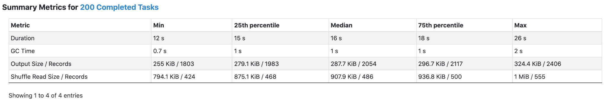
We can see that the max duration of a task is way bigger than the 75th percentile. It means that some tasks take much more time to finish than others. If we sort the tasks by duration, it turns out that it’s not a single outlier that took 26 seconds, but a recurring problem.

Usually, there can be two reasons for the task duration skew in repartitioned by key dataframe: either distribution of the data is not homogeneous by key and some partitions are much bigger than others, or there are some differences in data that make executors more time to process these partitions. There can be other reasons, like problems with the machine itself or competition for the resources when several jobs are running simultaneously on one cluster. We use Glue to avoid these kinds of problems. Since so far it worked, we decided to focus on data distribution and processing time for data associated with different keys.
First, we checked the distribution of the data by keys. For that, we can take a look at the Shuffle Read Size / Records column.
It looks pretty decent. The difference between the maximum size of the partition and the 75th percentile is around 10%, whereas the duration differs by 40%. So it is likely that the problem is that some of the partitioning keys contain data that take more time to process than others. We needed to look for transformations that take a disproportionately large amount of time. But even before that, we can change something to mitigate the problem.
Luckily enough, our partitioning column has a high cardinality of keys. So we can split the dataframe into more partitions, and the distribution of hard-to-process keys will become more even across the partitions. We should take into account, however, that a large number of partitions bring more overhead on management for Spark master. Also, partitions should be of a reasonable size. Empirically we figured out that locally for the fraction of data 400 partitions did the trick. For the production environment 2000 partitions of 20MB each worked well.
It is worth saying that in the production environment optimization will be even more significant. Let’s say we run the job with default configuration on 100 standard workers, then we have 200 partitions and 200 executors with 2 cores each (2 executors per worker with 4 cores). It means that each executor is working on their piece of data, and once they are finished, they don’t have anything to do and will wait until other executors finish their tasks. It can be a long time if some tasks are processed faster than others. With the new number of partitions, we could certainly utilize resources better.
Bingo! This small adjustment helped us to double the performance. But the stage was still taking too long for processing that amount of data. We decided to find the bottleneck.
Join Xomnia's Data & Drinks event about the latest trends in the world of AI. Click here.
Looking for the bottleneck...
The time had come for us to dive into the code. From here, there are infinite opportunities and hypotheses to check. Therefore, we need to bring the number of options down by asking questions. The most important one is which transformation takes so long.
Unfortunately, it’s not easy to profile separate pieces of code executed as one stage in Spark. Simple profiling wouldn’t work because Spark uses lazy evaluation, and nothing gets processed until Spark encounters an action instruction. All the functions in between reading data and action are executed instantly. To overcome this, we include dataframe.cache().count() instructions in the workflow. It splits executed transformations into different stages that can be observed from Spark UI. No doubt, this messes up the estimation because cache and count instructions affect execution in various and unpredictable ways. But it’s usually enough to identify the slow code in the workflow in case it is much slower than everything else around.
This time we were lucky. We could quickly identify the piece of code that took pretty much all the time on the stage. Without going too much into details, the code translated numbers between number systems several times, checked a couple of conditions, and reversed bits of numbers if needed. It has also done so for a few dozens of columns in a loop. Without much effort, we reduced the amount of a number system translations. We also made conditions smarter by using features of the binary representation of numbers.
After this, execution time has improved. The result was good but not outstanding. We won only 5-10%.
Spark UI before the optimization ...
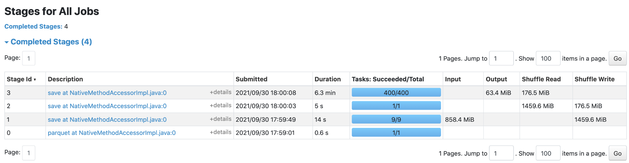
... and after
The bit-flip operation also caught our attention. It was implemented as a Spark function translate applied to a string representation of a binary number. It was a clear candidate for optimization because bit strings are long, and string operations are generally expensive. We thought that there should be a way to do bit-flips faster with built-in bitwise operations. Unfortunately, it didn’t work. We managed to employ bitwiseNOT, but we still had to apply pattern matching on strings because the bitwiseNOT operation in Spark also flips leading zeros (as it should). We needed it to flip only significant bits and didn’t find another way to do it in Spark 2.4. The quick experiment showed that the version with bitwiseNOT + regexp_replace works slower than just translate operation.
At this point, with the applied optimizations, we already reduced the execution time by 50%, so we could stop. Saving 50% of running costs is already a decent result. But there still was a feeling that something was off. Then we noticed two interesting things …
Know more about Xomnia, the leading AI consultancy in the Netherlands
Bonus: what happens when whole stage code generation fails in Spark?
The first clue we’ve noticed was that the stage with a long duration also emitted ERROR logs from CodeGenerator
2021-08-31 16:20:09 ERROR CodeGenerator:91 - failed to compile: org.codehaus.janino.InternalCompilerException: Compiling "GeneratedClass": Code of method "processNext()V" of class "org.apache.spark.sql.catalyst.expressions.GeneratedClass$GeneratedIteratorForCodegenStage4" grows beyond 64 KB
org.codehaus.janino.InternalCompilerException: Compiling "GeneratedClass": Code of method "processNext()V" of class "org.apache.spark.sql.catalyst.expressions.GeneratedClass$GeneratedIteratorForCodegenStage4" grows beyond 64 KB
at org.codehaus.janino.UnitCompiler.compileUnit(UnitCompiler.java:382)
at org.codehaus.janino.SimpleCompiler.cook(SimpleCompiler.java:237)
at org.codehaus.janino.SimpleCompiler.compileToClassLoader(SimpleCompiler.java:465)
at org.codehaus.janino.ClassBodyEvaluator.compileToClass(ClassBodyEvaluator.java:313)
...
The error was followed by the warning from WholeStageCodefenExec
at org.codehaus.janino.UnitCompiler.compile(UnitCompiler.java:406)
at org.codehaus.janino.UnitCompiler.compileUnit(UnitCompiler.java:378)
... 51 more
2021-08-31 16:20:09 WARN  WholeStageCodegenExec:66 - Whole-stage codegen disabled for plan (id=4):
...
Well, we knew that Spark generates Java code for the execution of the stage. StackOverflow offered to put a cache instruction before the stage to get rid of the error. But the job didn't fail, and it looked like Spark handled the situation pretty well. We decided to leave everything as is. Also, the solution with cache didn’t change anything. And then, we looked at the execution plan again.
At the current stage, we had a loop creating 2 dozen columns from a base column. What puzzled us was that the execution plan referred directly to the base column 8 times for every new column created. Be the plan executed as-is, some transformations would be applied 4 times, others 8, and some others - those which are common for all the columns - 200 times. It would be an immense waste! Ideally, we’d like Spark to optimize it for us, calculate intermediate results once, cache, and reuse it.
*(4) Project [CASE WHEN ((cast(conv(concat(element_at(split(base_col#9680, :), 5), element_at(split(base_col#9680, :), 6)), 16, 10) as int) <= 32767) && (cast(conv(concat(element_at(split(base_col#9680, :), 5), element_at(split(base_col#9680, :), 6)), 16, 10) as int) > -1)) THEN cast(cast(conv(concat(element_at(split(base_col#9680, :), 5), element_at(split(base_col#9680, :), 6)), 16, 10) as int) as double) ELSE -(cast(conv(regexp_replace(bin(cast(~cast(conv(concat(element_at(split(base_col#9680, :), 5), element_at(split(base_col#9680, :), 6)), 16, 10) as int) as bigint)), ^[1]+, ), 2, 10) as double) + 1.0) END AS col1#12353, ...These two observations combined made us wonder whether optimizations do not apply when code generation fails. It turned out that this indeed happened. Whole-Stage Code Generation creates one Java function from the whole stage. It reduces the number of function calls which allows keeping the data in the processor memory longer. It also applies other various optimizations. For more details, check the talk from Databricks or the original article Efficiently Compiling Efficient Query Plans for Modern Hardware written by Thomas Neuman.
We decided to separate the common part of transformation for all the produced columns and give Spark an explicit instruction that this data shall be cached after calculation. Apparently, cache instruction also splits the code created by Whole-Stage Code Generation in two parts, transformations applied before cache and after it, so that intermediate results could be cached. This way, Java class can become smaller and fit in 64KB limitation.
Checking the execution plan again, we can see that instead of applying the same functions on the base column, we use intermediate cached columns. The errors and warnings are also gone from the logs
+- *(4) Project [CASE WHEN ((intermediate_col_1#606 <= 32767) && (intermediate_col_1#606 > -1)) THEN cast(intermediate_col_1#606 as double) ELSE -(cast(conv(regexp_replace(bin(cast(~intermediate_col_1#606 as bigint)), ^[1]+, ), 2, 10) as double) + 1.0) END AS intermediate_col_1#3524, ...
...
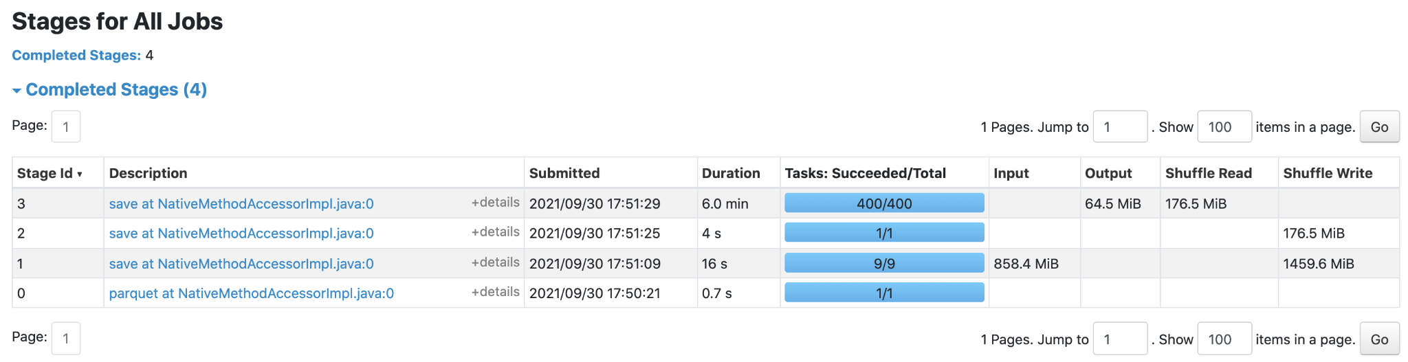
+- *(1) Project [cast(conv(concat(element_at(split(base_col#405, :), 5), element_at(split(base_col#405, :), 6)), 16, 10) as int) AS intermediate_col_1#606, ...But what is more important is that execution time was reduced by a factor of 6!
Spark UI before the optimization ...
... and after
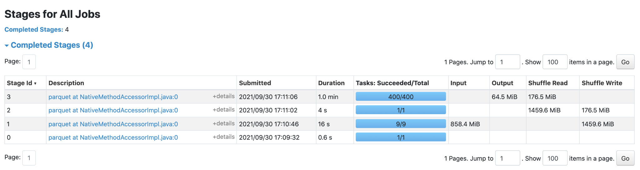
Unfortunately, we couldn’t reproduce the same result in the production environment. The whole intermediate dataframe didn’t fit in memory, and Spark spilled it on disk. This operation and management of the dataframe on disk gave quite some overhead, so this optimization gave us a smaller improvement of performance - by a factor of 3. Success!
Don't miss Xomnia's latest business cases and blogs. Subscribe to our newsletter.
Conclusions
Thank you for going through this story together with us. In the last section, we’d like to reflect on the result and process.
First of all, all optimizations together helped us make the job 6 times faster or, in other words, saved us 83% of resources. It’s a stellar result, but we were “lucky” to have space for such optimization. It doesn’t always go the same way. However, we think that the approach we take when optimizing Spark workflows is simple and usually gives good results in a short amount of time, so we are glad to share it.
Second, at Xomnia, we frequently encounter the compromise between high delivery speed and low infrastructure costs. Managed services, like Glue, allow teams to move faster and spend fewer resources on support, but they also cost more. In this article, we showed, how with a bit of optimization, the costs of Glue can be brought down significantly, which makes Glue more accessible for the teams focused on rapid delivery.
We encourage teams to make decisions on using managed services considering the use case and environment requirements. As a rule of thumb, at Xomnia, we start working with managed services and make the system ready for the infrastructure change by separating infrastructure concerns from the domain logic of an application. This way, we deliver value as soon as possible, which creates credibility for the team to extend the solution, improve it and reduce the costs if needed in one way or another.