If you’re an analytics engineer – someone comfortable with SQL and also into visualising data – there’s a good chance you’ve noticed Power BI has been making inroads into the business intelligence landscape.

You’ve probably also noticed that there are a lot more data sources out there these days. Maybe you’re using a data warehouse you built yourself, maybe you’re leveraging a central data lake, and maybe you’re also using some third-party datasets specific to your business unit’s needs. Chances are that SQL is still an important skill to have when combining all these sources.

So your data loading and transformations are all done and now comes the easy part, right? You just have to connect Power BI to your data and slap some dashboards together. Usually this starts off easily, but as your reporting users get more sophisticated in their demands, they think of news ways they want to slice and dice their data, and more exotic ways in which they’d like to visualise it.

This is when your SQL experience starts to get in the way. You know how to query the data using SQL, but creating Power BI slicers and measures just doesn’t seem intuitive, and the examples you find in forums aren’t too difficult to adapt, but you’re not sure how they came up with them.

In this blog post, Michael Moore would like to demonstrate some of the fundamental differences between SQL and DAX, and how to re-tune your thought processes to become more productive with Power BI.

SQL vs DAX: The Low Down

Structured Query Language (SQL) and Data Analysis Expressions (DAX) are both tools for working with data, but they serve distinct purposes and operate under different paradigms.

1. Declarative versus Functional

• SQL describes what you want, not how to get it.

-- SQL example
SELECT department, AVG(salary)
FROM employees
GROUP BY department

• DAX is based on functions and filters.

-- DAX example
Department = SELECTEDVALUE(Employees[Department])
AverageSalary = AVERAGE(Employees[Salary])

2. Rows versus Columns

SQL: Primarily row-based and designed for transactional databases. Queries retrieve and manipulate sets of rows and their intersection.

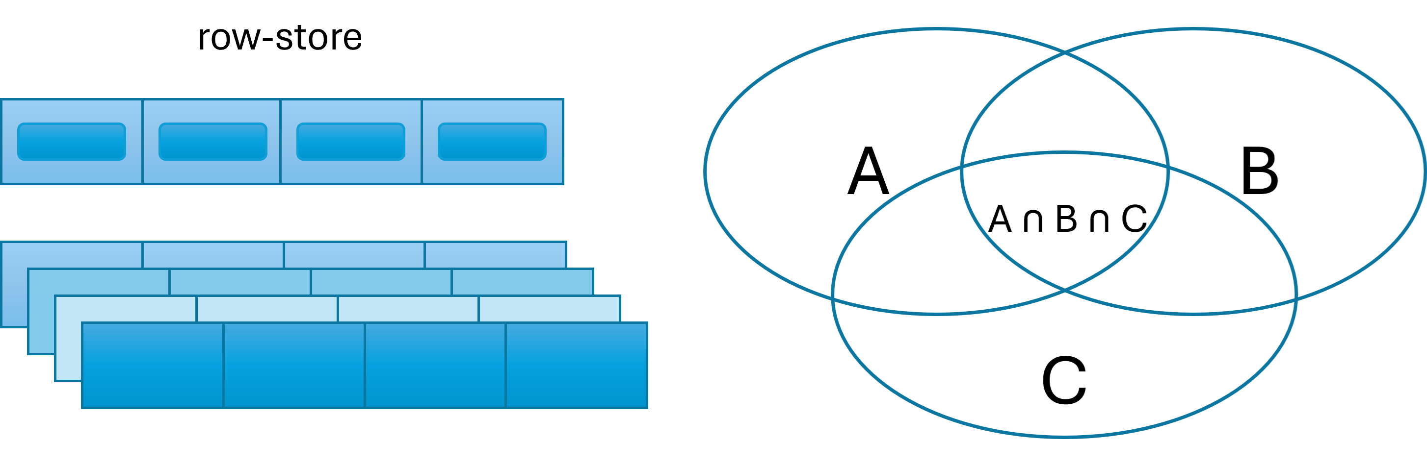
• DAX: Column-based and optimised for data retrieval. Calculations operate by default on entire columns rather than individual rows using vectors.
  

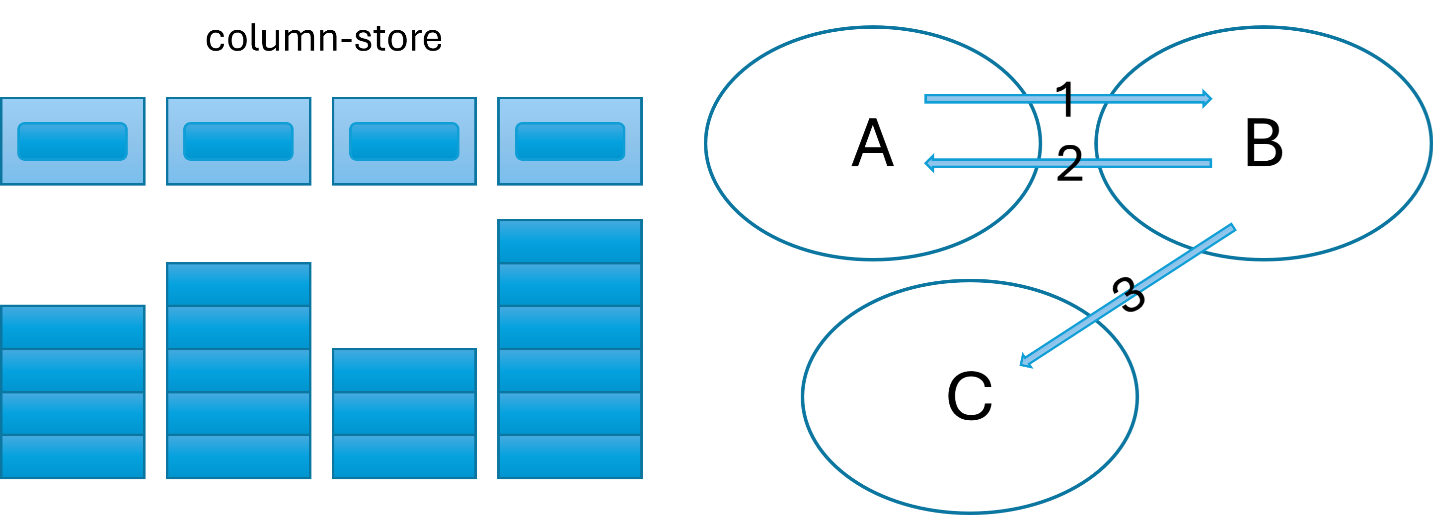
3. Independence versus Context

• SQL: Queries declare the conditions and joins of what you need, with logic that is evaluated independently of other queries.
• DAX: Evaluations depend on row and filter context, meaning results vary depending on applied filters and aggregations.

This last bullet point is key to answering the question of why Microsoft didn’t just stick with SQL: Calculations using DAX are dynamic. In SQL, you bake a cake and slice it. In DAX, you slice the cake while it’s still in the oven. This results in each slice having its own baking steps, which are implemented using two key concepts: context and filters.

Let’s look at some examples of how things are done in DAX measures to help shift your mindset.

Pitfalls SQL Experts Fall into with DAX Measures

1. Using Multiple Columns in Aggregate Functions

• Unlike SQL, where multiple columns can be used directly in aggregations, DAX requires iteration on expressions over rows, by switching to "row context".
• Solution: Use row context functions SUMX(), AVERAGEX(), COUNTX() instead of simple aggregators like SUM(), AVERAGE(), COUNT() when dealing with multiple columns.

Example of SQL multi-column aggregation

-- Calculate the total of all product sales
SELECT SUM(Sale.Quantity * Sale.Price) AS TotalRevenue
FROM Sale

Incorrect equivalent DAX aggregation using SUM()

// Generates an error because SUM() only allows columns, not expressions
TotalRevenue = SUM(Sale[Quantity] * Sale[Price])

// This will work but isn’t what we want
TotalQuantity = SUM(Sale[Quantity]) * SUM(Sale[Price])

We will shift from the standard column context to a row context using SUMX(), which allows expressions:

SUMX(<table>, <expression>)

Correct equivalent DAX aggregation using SUMX()

TotalRevenue = 
SUMX(                             // switch to row context
    Sale,                         // for each row in Sale
    Sale[Quantity] * Sale[Price]  // calculate this expression
)

The SUMX() function switches from column to row context where we can iterate over each record.

2. Thinking in Joins instead of Relationships

• SQL relies heavily on JOIN operations to combine tables.
• DAX leverages predefined relationships between tables in your semantic model.
• Solution: Use the RELATED() function instead of explicit joins.

Example of SQL JOIN

-- Calculate the total of all product sales
SELECT SUM(Sale.Quantity * Product.Price) AS TotalRevenue
FROM Sale
JOIN Product ON Sale.ProductID = Product.ProductID

The function we need returns a single value from the column specified, that is related to the current row:

RELATED(<column>

Equivalent DAX join using RELATED()

// Using RELATED() to sum two columns from related tables
TotalRevenue = 
SUMX(
    Sale,                                     // for each row in Sale
    Sale[Quantity] * RELATED(Product[Price])  // calculate this expression
)

Notice how RELATED() retrieves a value from Product? We iterate over the many rows in Sale, because that allows us to create an expression with one Price per Quantity.

3. Returning Result Sets from Measures

• SQL can happily return result sets with multiple rows and columns but DAX measures must return one value.
• Solution: Use a row context function like CONCATENATEX() to aggregate multiple values.

Example of SQL DISTINCT

-- Retrieve a list of unique product names
SELECT DISTINCT Product.ProductName
FROM Product

DAX has the following function to retrieve a distinct list of values:

VALUES(<TableNameOrColumnName>)

Incorrect Equivalent DAX measure using VALUES()

// Use VALUES() to create a one-column table of unique product names
ProductList = VALUES('Product'[ProductName])

Error: A table of multiple values was supplied where a single value was expected

The problem is that VALUES() returns a table, which cannot be used as a return value.

To fix the error, we need to use CONCATENATEX() with the syntax:

CONCATENATEX(<table>, <expression>, <delimiter>)

Correct Equivalent DAX measure using VALUES() and CONCATENATEX()

// Corrected measure with iterator to concatenate values
ProductList = 
RETURN 
CONCATENATEX(	
    VALUES('Product'[ProductName]),  // one column table of product names
    [ProductName],                   // column name expression
    ", "
)

4. Forgetting Filter and Row Context

• In SQL, set and row filters are explicitly defined in the WHERE and GROUP BY clauses, and calculations always work with the full dataset that matches the conditions.
• DAX evaluates expressions dynamically based on row and filter context.
• Solution: Understand how slicers, a visual’s x-axis and functions like CALCULATE(), ALL(), and SELECTEDALL() modify the context.

As said before, DAX slices the cake in the oven, so depending on the filter context being applied, the TotalRevenue measure created above can be the sum of one row, multiple rows, or all rows.

What this means is that if you use the TotalRevenue measure on a KPI visual, you will see the sum of all sales ever made, whereas in a bar chart with year on the X-axis, the same measure will calculate the sum per year.

If you then add a page slicer to filter sales by the department, then both the KPI and bar chart will only show sales for that department.

So what if you want to set a filter context that’s not in a slicer? That’s what CALCULATE() is for. Take the situation where we want to limit the sales figures to 2023.

Example of SQL WHERE filter

SELECT SUM(Sale.Quantity * Product.Price) AS TotalRevenue
FROM Sale
JOIN Product ON Sale.ProductID = Product.ProductID
WHERE YEAR(Sale.TransactionDate) = 2023

To simulate the WHERE clause we need the following DAX function:

CALCULATE(<expression>[, <filter1>, <filter2>,...])

Equivalent DAX filter using CALCULATE()

TotalRevenue2023 =
CALCULATE(
    SUMX(                                         // expression
        Sale,		
        Sale[Quantity] * RELATED(Product[Price])
    ),
    YEAR(Sale[TransactionDate]) = 2023            // filter
)

And what about when we want to ignore any filters and calculate using all rows? Intuitively, there is a function called ALL(). In the following scenario, I will calculate the percentage of each year’s sales from the combined total.

Example of SQL percentage calculation

WITH RevenueData AS (
    SELECT 
        Sale.TransactionDate,
        Sale.Quantity * Product.Price  AS Revenue
    FROM Sale
    JOIN Product ON Sale.ProductID = Product.ProductID
),
AllYears AS (
    SELECT SUM(Revenue)                AS TotalRevenue
    FROM RevenueData
)
SELECT 
    YEAR(TransactionDate)              AS "Year",
    SUM(Revenue)                       AS TotalYearRevenue,
    SUM(Revenue) / ay.TotalRevenue     AS PercOfAllYearRevenue
FROM RevenueData
JOIN AllYears ay ON 1=1  -- same as cross-join
GROUP BY YEAR(TransactionDate)

SQL Result Set

Year	TotalYearRevenue	PercOfAllYearRevenue
2022	13500	40
2023	15600	45
2024	5000	15

Equivalent DAX percentage calculation using ALL()

PercentageOfTotalRevenue =
VAR AllYearTotalSales =
    SUMX(
        ALL(Sale),                                // ignore any filters on Sale
        Sale[Quantity] * RELATED(Product[Price])
    )
VAR TotalSales =
    SUMX(
        Sale,                                     // only look at filtered rows
        Sale[Quantity] * RELATED(Product[Price])
    )
RETURN DIVIDE(TotalSales, AllYearTotalSales)

The ALL() function has the syntax:

ALL( <table> | <column> )

When used with a function like SUMX() it allows us to ignore any filters in place whereas the second SUMX() function continues to use the current filter context.

FYI. The DIVIDE() function returns BLANK() on division by zero.

Next we are really going to dive into the weeds of Power BI by looking at the SQL RANK() function and its equivalent RANKX() in DAX.

Example of SQL RANK window function

WITH RevenuePerProduct AS (
    -- Sum the revenue per product
    SELECT Product.ProductName, 
        SUM(Sale.Quantity * Product.Price) AS ProductRevenue
    FROM Sale
    JOIN Product ON Sale.ProductID = Product.ProductID
    GROUP BY Product.ProductName
)
-- Rank the revenue per product starting with 1 as the highest
SELECT 
    ProductName, 
    ProductRevenue,
    RANK() OVER (
        PARTITION BY ProductName
        ORDER BY ProductRevenue DESC
    ) AS ProductRank
FROM RevenuePerProduct

SQL Result Set

ProductRevenue	ProductRevenue	ProductRank
Sofa	25000	1
Radio	3600	2
Headphone	3000	3
Blender	2500	4

The basic DAX syntax for RANKX() is:

RANKX(<table>, <expression>)

It works by following three steps:

1. Build a sorted list by evaluating the expression over the table.
2. Calculate the current row’s value in the given context.
3. Find where the value (from Step 2) fits in the sorted list (from Step 1).

Incorrect equivalent DAX using RANKX()

ProductRank = 
RANKX(	
    ALL('Product'), 	
    SUMX(
        Sale, 
        Sale[Quantity] * RELATED(Product[Price])
    )
)

The DAX above would appear to be good. ALL() is used so that each product's revenue is ranked against a list of all others. From the result below, however, you can see that this is not what we want.

Unfortunately, ALL() creates a row context where both step 1 and step 2 are calculated for all rows, causing all products to have the same total revenue.

The solution? We need to use the CALCULATE() function to shift the row context into a filter context. This will ensure that the step 2 revenue is computed for just one product.

Improved equivalent DAX using RANKX() and CALCULATE()

ProductRank = 
RANKX(
    ALL('Product'),
    CALCULATE(       // use per row filter context created by RANKX()
        SUMX(
            Sale,
            Sale[Quantity] * RELATED(Product[Price])
        )
    )
)

Alternatively, we can also use the TotalRevenue measure that we created before, as all measures are implicitly surrounded by CALCULATE().

Improved equivalent DAX using RANKX() and measure

ProductRank =
RANKX(
    ALL('Product'),
    [TotalRevenue]   // measure defined previously with implicit CALCULATE()
)

Everything looks good now – well almost.

Firstly, the total has a rank too, which looks a bit odd. Secondly, and more critically, the rank ignores the slicer filter, due to the ALL() that we used. We can solve these issues with the ISINSCOPE() and ALLSELECTED() functions.

Correct equivalent DAX ranking using ISINSCOPE() and ALLSELECTED()

ProductRank = 
IF(
    ISINSCOPE('Product'[ProductName]),
    RANKX(
        ALLSELECTED('Product'),   // use filter context created by slicer
        TotalRevenue
    )
)

That looks better. ISINSCOPE() limits evaluation to rows where ProductName exists (“Total” is not one of them), and ALLSELECTED() ranks according to the filter context of the slicer.

5. Forgetting cross-filter JOIN direction

• In SQL, filters limit the records available in all joined tables.
• Power BI models filter by default, only on the many-side of relationships.
• Solution: Understand how to modify cross-filter directions in the semantic model or use the CALCULATETABLE() and FILTER() functions to modify the filter context.

Let’s look at our sales revenue again, along with the Product List measure we created before.

DAX measure using VALUES() and CONCATENATEX()

// DAX measure that retrieves all product names
Product List = 
CONCATENATEX(
    VALUES('Product'[ProductName]),  // get table of product names
    [ProductName],                   // use column value	
    ", "                             // specify list separator
)

Now we know that not all products are sold every year, so why is every product name appearing? The reason is that only sale records are contained in the filter context. Our semantic model only allows filtering on the many-side, not the one-side.

Now the easiest way to fix this is to click on the relationship properties and change the cross-filter direction to work in both directions.

But for educational purposes, let’s use some DAX functions to get the result that we want.

Our goal is to enforce the filtering we need by going through a many-side relationship. If we use the previously demonstrated technique, then RELATED() seems like a good candidate.

DAX measure using CONCATENATEX() and RELATED()

// DAX measure to retrieve only selected products
Product List =
CONCATENATEX(
    'Sale',                           // force context to go through Sale	
    RELATED('Product'[ProductName]),
    ", "
)

This is close but unfortunately we have duplicates, especially on the total row, as CONCATENATEX() has no feature to remove duplicates like VALUES().

Instead we can use a function with the following syntax:

CALCULATETABLE(<table>, <table or filter expression>)

It returns a set of rows based on the expression, for all rows specified by the table filter. This way we can return only the product rows that match the sale context. Because each row in Product is naturally distinct, we remove duplicates.

Correct DAX measure using CONCATENATEX(), CALCULATETABLE() and VALUES()

// DAX measure that retrieves a distinct list of product names
Product List =
CONCATENATEX(
    CALCULATETABLE(
        'Product',          // give me all the rows from Product		
        'Sale'              // that are related to the Sale context
	),
	'Product'[ProductName],	
    ", ",	
    'Product'[ProductName]  // optional: sorts alphabetically
)

Hooray! We have achieved our desired result.

Another way to implement this is via the FILTER() function with the following syntax:

FILTER(<table>, <filter expression>)

Once again, we are forcing the context to go through Sale to ensure we only see the product names we need.

Correct DAX measure using CONCATENATEX(), FILTER() and VALUES()

// DAX measure that retrieves a distinct list of product names
Product List =
CONCATENATEX(
    FILTER(         // retrieve product rows product ID match the Sale context
        'Product',
        'Product'[ProductID] IN VALUES(Sale[ProductID])	
    ),	
    'Product'[ProductName],	 // Product names table is already unique
    ", "
)

A third technique involves using the SELECTCOLUMNS() function along with DISTINCT().

The latter function has the following syntax:

SELECTCOLUMNS(<table>, <assigned name>, <expression>)

Correct DAX measure using CONCATENATEX(), DISTINCT() and SELECTCOLUMNS()

// DAX measure that retrieves a distinct list of product names
Product List =
CONCATENATEX(
    DISTINCT(                 // make selected column distinct
        SELECTCOLUMNS(
            Sale,             // for each record in Sale context
            "Product_Name",   // create a column called Product_name
            RELATED('Product'[ProductName])  // from the ProductName table
        )
    ),
    [Product_Name],           // use the column defined earlier
    ", "
)

Working with Large Language Models (LLM’s)

Using services like ChatGPT and Claude are great tools to boost your productivity. Here are some tips and tricks that I’ve learnt to help you get the right result.

Topic	Description	Prompt Example
Measure or calculated column	Specify if you want a DAX measure or calculated column, they often work differently.	Please generate a DAX measure that sums Sales[Quantity] * Product[Price]
SQL translation	Provide the SQL that works and ask it to convert it.	Translate this SQL into a DAX measure: SELECT SUM(Sales.Quantity * Product.Price) AS TotalRevenue FROM Sale
Relationship definition	First describe the 1-to-many relationships between your tables.	Assuming I have a Product table with a 1-to-many relationship to a Sales table, please generate a DAX measure that…
Error messages	Paste in any Power BI error messages you receive along with the broken code.	Why does my DAX measure: ProductList = VALUES('Product'[ProductName]) generate the following error? Error: A table of multiple values was supplied where a single value was expected
Sample data	Upload some sample data first using CSV files, JSON, or copy/paste the data from Excel. You can also upload screenshots of data or semantic models.	Here’s my Sales and Product data. Please generate a DAX measure that…

Cheat Sheet and Final Thoughts

SQL Concept	DAX Equivalent
SUM(column * column)	SUMX(table, column * column)
JOIN	RELATED() or CALCULATETABLE() with the relationship one-side table. FILTER() with VALUES() on the many-side table.
WHERE	CALCULATE(), FILTER() or CALCULATETABLE() to add explicit filter ALL() to ignore filter context ALLSELECTED() to explicitly use filter context
GROUP BY	Implicit in measure/visual/filter context
DISTINCT	DISTINCT() and SELECTCOLUMNS(), or VALUES() as parameter of CONCATENATEX()
WITH (common table expression) and sub-queries	VAR, or Build and reference separate measures
RANK	RANKX() with ALLSELECTED() and CALCULATE()

There’s a lot to get your head around with the examples above, and changing your way of thinking doesn’t happen overnight. However, I hope that this shows you how DAX works differently to SQL and helps set you on your way to becoming proficient at creating measures with DAX in Power BI.