Ritchie is a Data Scientist & Big Data Engineer at Xomnia. Besides working at Xomnia, he writes blogs on his website about all kinds of machine- and deep learning topics, such as: “Assessing road safety with computer vision” and “Computer build me a bridge”. Expect more interesting blogs from Ritchie in the future.
Introduction
Last post I’ve described the Affinity Propagation algorithm. The reason why I wrote about this algorithm was that I was interested in clustering data points without specifying k, i.e. the number of clusters present in the data.
This post continues with the same fascination, however, now we take a generative approach. In other words, we are going to examine which models could have generated the observed data. Through Bayesian inference, we hope to find the hidden (latent) distributions that most likely generated the data points. When there is more than one latent distribution we can speak of a mixture of distributions. If we assume that the latent distributions are Gaussians than we call this model a Gaussian Mixture model.
First, we are going to define a Bayesian model in Edward to determine a multivariate Gaussian mixture model where we predefine k. Just as in k-means clustering we will have a hyperparameter k that will dictate the amount of clusters. In the second part of the post, we will reduce the dimensionality of our problem to one dimension and look at a model that is completely nonparametric and will determine k for us.
Dirichlet Distribution
Before we start with the generative model, we take a look at the Dirichlet distribution. This is a distribution of distributions and can be a little bit hard to get your head around. If we sample from a Dirichlet we’ll retrieve a vector of probabilities that sum to 1. These discrete probabilities can be seen as separate events. A Dirichlet distribution can be compared to a bag of badly produced dice, where each dice has a totally different probability of throwing 6. Each time you sample a dice from the bag you sample another probability of throwing 6. However, you still need to sample from the dice. Actually throwing the dice will lead to sampling the event.
The Dirichlet distribution is defined by:

where

This distribution has one parameter α that influences the probability vector that is sampled. Let’s take a look at the influence of α on the samples. We can best investigate the Dirichlet distribution in three dimensions; θ=[θ1,θ2,θ3]. We can plot every probability sample θ as a point in three dimensions. By sampling a lot of distribution points θ, we will get an idea of the Dirichlet distribution Dir(α).
If we want to create a Dirichlet distribution in three dimensions we need to initialize it with α=[α1,α2,α3]. The expected value of θ becomes:

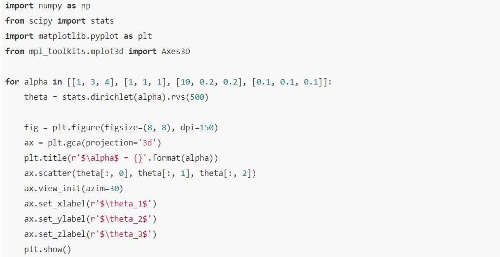
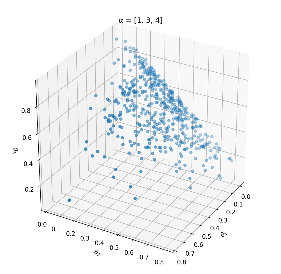
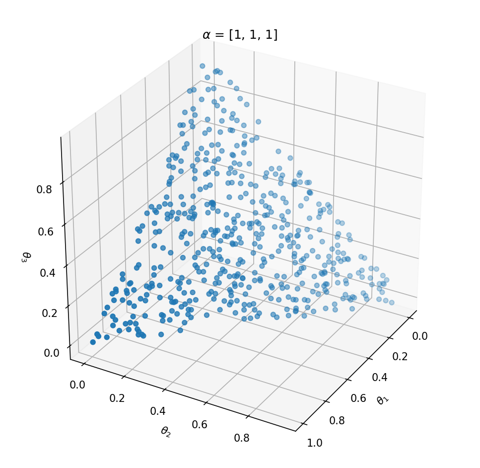
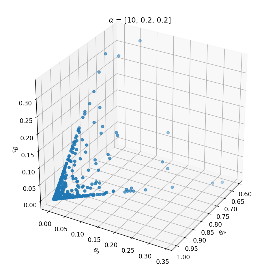
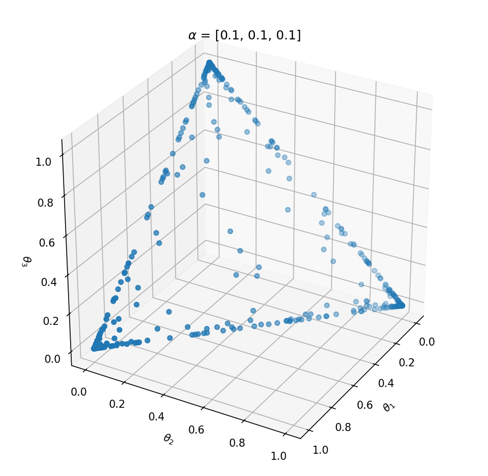
Above the underlying distribution of Dir(α) is shown by sampling from it. Note that α=[10,0.2,0.2] leads to high probability of P(α1) close to 1 and that α=[1,1,1] can be seen as uniform Dirichlet distribution, i.e. that there is an equal probability for all distributions that suffices ∑ki=1
Clustering with generative models
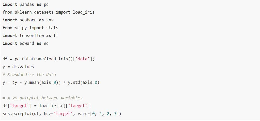
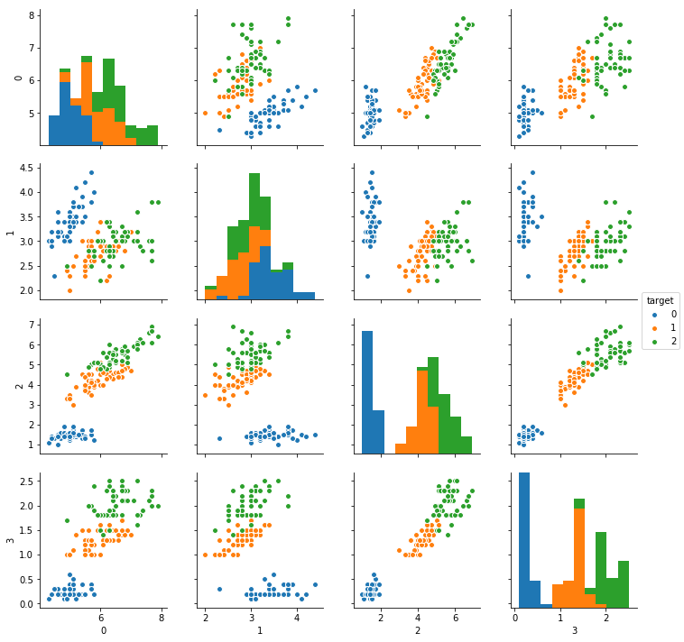
Now, we have had a nice intermezzo of Dirichlet distributions, we’re going to apply this distribution in a Gaussian Mixture model. We will try to cluster the Iris dataset. This is a dataset containing 4 columns of data gathered from 3 different types of flowers.
Gaussian Mixture
A Gaussian Mixture model is the Mother Of All Gaussians. For column 0 in our dataframe it is the cumulative of the histograms of the data labels.
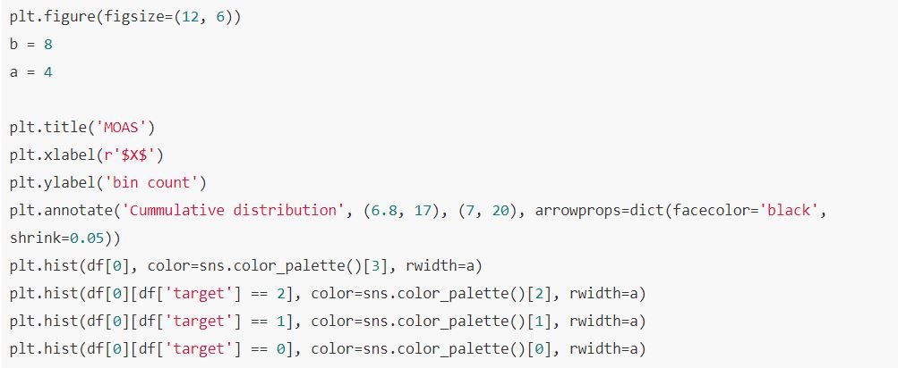
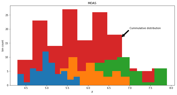
Of which we obtain a dataset without labels. Moreover, what we can observe from the real world, is the single red distribution. However, we know now that the data actually is produced by the 3 latent distributions, namely three different kinds of flowers. The red observed distribution contains a mixture of the hidden distributions. We could model this by choosing a mixture of 3 Gaussian distributions
However, the integral of a Gaussian distribution is equal to 1 (as a probability function should be). If we combine various Gaussians we need to weigh them so the integral will meet the condition of being equal to 1.

We could of course scale the mixture of Gaussian by weights summing to 1. Here comes the Dirichlet distribution in place. Every sample from a Dirichlet sums to one and could be used as weights to scale down the mixture of Gaussian distributions.
The final generative model can thus be defined by:

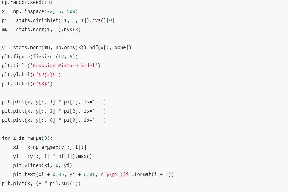
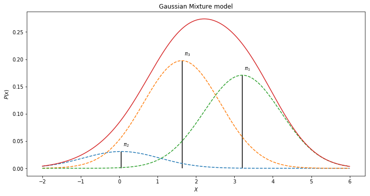
where π are the weights drawn from Dir(α). One such mixture model for the histogram above for instance could look like:
. One such mixture model for the histogram above for instance could look like:
Interested in reading the full blog?
For the full blog, visit Ritchie’s website to read about:
– Uncertainty
– Cluster assignment
– Dirichlet Process
– Nonparametric clustering
– Dirichlet Process Mixtures in Pymc3
– Inferred k
– And the conclusion
Or read the previous blog about the Affinity Propagation algorithm.
(c) 2018 Ritchie Vink.


